5.7 GLMakie.jl

CairoMakie.jl 满足了所有关于静态 2D 图的需求。 但除此之外，有时候还需要交互性，特别是在处理 3D 图的时候。 使用 3D 图可视化数据是 洞察 数据的常见做法。 这就是 GLMakie.jl 的用武之地，它使用 OpenGL 作为添加交互和响应功能的绘图后端。 与之前一样，一幅简单的图只包括线和点。因此，接下来将从简单图开始。因为已经知道布局如何使用，所以将在例子中应用一些布局。

5.7.1 散点图和折线图

散点图有两种绘制选项，第一种是 scatter(x, y, z)，另一种是 meshscatter(x, y, z)。 若使用第一种，标记则不会沿着坐标轴缩放，但在使用第二种时标记会缩放， 这是因为此时它们是三维空间的几何实体。 例子如下：

using GLMakie
GLMakie.activate!()

function scatters_in_3D()
    seed!(123)
    xyz = randn(10, 3)
    x, y, z = xyz[:, 1], xyz[:, 2], xyz[:, 3]
    fig = Figure(resolution=(1600, 400))
    ax1 = Axis3(fig[1, 1]; aspect=(1, 1, 1), perspectiveness=0.5)
    ax2 = Axis3(fig[1, 2]; aspect=(1, 1, 1), perspectiveness=0.5)
    ax3 = Axis3(fig[1, 3]; aspect=:data, perspectiveness=0.5)
    scatter!(ax1, x, y, z; markersize=50)
    meshscatter!(ax2, x, y, z; markersize=0.25)
    hm = meshscatter!(ax3, x, y, z; markersize=0.25,
        marker=FRect3D(Vec3f(0), Vec3f(1)), color=1:size(xyz)[2],
        colormap=:plasma, transparency=false)
    Colorbar(fig[1, 4], hm, label="values", height=Relative(0.5))
    fig
end
scatters_in_3D()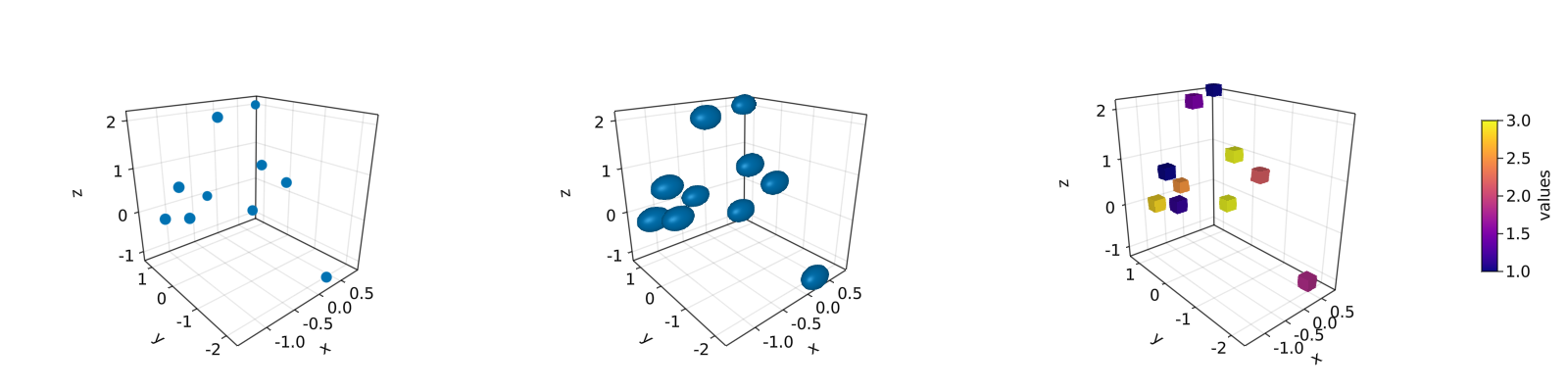

另请注意，标记可以是不同的几何实体，比如正方形或矩形。另外，也可以为标记设置 colormap。 对于上面位于中间的 3D 图，如果想得到获得完美的球体，那么只需如右侧图那样添加 aspect = :data 参数。 绘制 lines 或 scatterlines 也很简单：

function lines_in_3D()
    seed!(123)
    xyz = randn(10, 3)
    x, y, z = xyz[:, 1], xyz[:, 2], xyz[:, 3]
    fig = Figure(resolution=(1600, 400))
    ax1 = Axis3(fig[1, 1]; aspect=(1, 1, 1), perspectiveness=0.5)
    ax2 = Axis3(fig[1, 2]; aspect=(1, 1, 1), perspectiveness=0.5)
    ax3 = Axis3(fig[1, 3]; aspect=:data, perspectiveness=0.5)
    lines!(ax1, x, y, z; color=1:size(xyz)[2], linewidth=3)
    scatterlines!(ax2, x, y, z; markersize=50)
    hm = meshscatter!(ax3, x, y, z; markersize=0.2, color=1:size(xyz)[2])
    lines!(ax3, x, y, z; color=1:size(xyz)[2])
    Colorbar(fig[2, 1], hm; label="values", height=15, vertical=false,
        flipaxis=false, ticksize=15, tickalign=1, width=Relative(3.55 / 4))
    fig
end
lines_in_3D()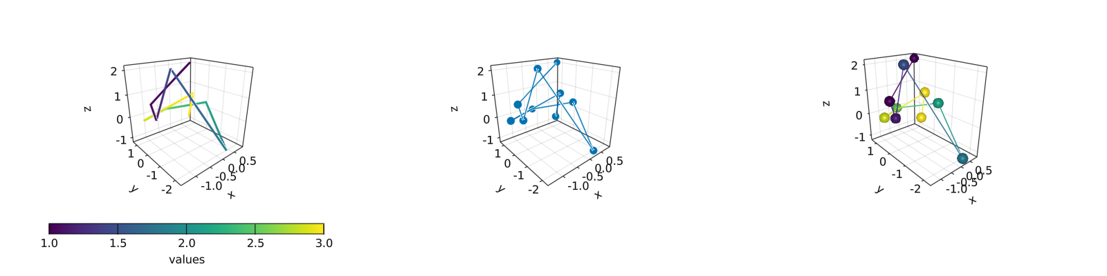

在 3D 图中绘制 surface， wireframe 和 contour 是一项容易的工作。

5.7.2 surface，wireframe，contour，contourf 和 contour3d

将使用如下的 peaks 函数展示这些例子：

function peaks(; n=49)
    x = LinRange(-3, 3, n)
    y = LinRange(-3, 3, n)
    a = 3 * (1 .- x') .^ 2 .* exp.(-(x' .^ 2) .- (y .+ 1) .^ 2)
    b = 10 * (x' / 5 .- x' .^ 3 .- y .^ 5) .* exp.(-x' .^ 2 .- y .^ 2)
    c = 1 / 3 * exp.(-(x' .+ 1) .^ 2 .- y .^ 2)
    return (x, y, a .- b .- c)
end

不同绘图函数的输出如下：

function plot_peaks_function()
    x, y, z = peaks()
    x2, y2, z2 = peaks(; n=15)
    fig = Figure(resolution=(1600, 400), fontsize=26)
    axs = [Axis3(fig[1, i]; aspect=(1, 1, 1)) for i = 1:3]
    hm = surface!(axs[1], x, y, z)
    wireframe!(axs[2], x2, y2, z2)
    contour3d!(axs[3], x, y, z; levels=20)
    Colorbar(fig[1, 4], hm, height=Relative(0.5))
    fig
end
plot_peaks_function()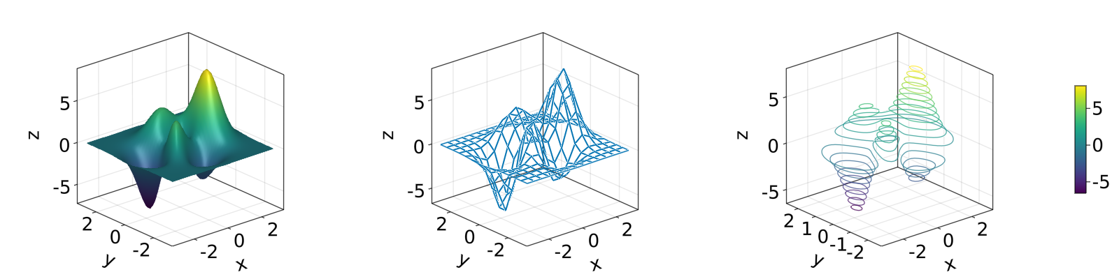

但是也可以使用 heatmap(x, y, z)，contour(x, y, z) 或 contourf(x, y, z) 绘图：

function heatmap_contour_and_contourf()
    x, y, z = peaks()
    fig = Figure(resolution=(1600, 400), fontsize=26)
    axs = [Axis(fig[1, i]; aspect=DataAspect()) for i = 1:3]
    hm = heatmap!(axs[1], x, y, z)
    contour!(axs[2], x, y, z; levels=20)
    contourf!(axs[3], x, y, z)
    Colorbar(fig[1, 4], hm, height=Relative(0.5))
    fig
end
heatmap_contour_and_contourf()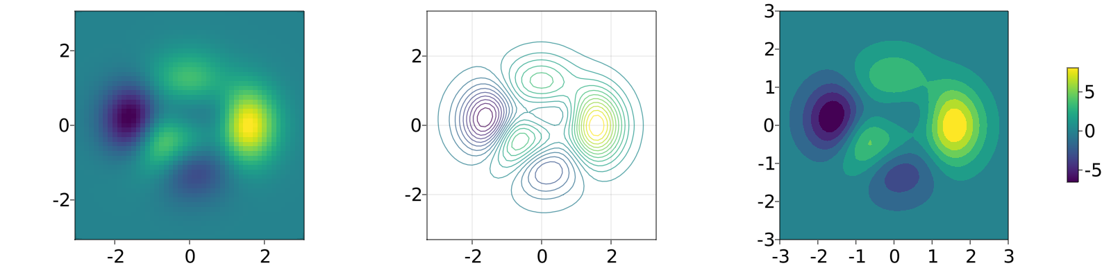

另外，只要将Axis 更改为 Axis3，这些图就会自动位于 x-y 平面：

function heatmap_contour_and_contourf_in_a_3d_plane()
    x, y, z = peaks()
    fig = Figure(resolution=(1600, 400), fontsize=26)
    axs = [Axis3(fig[1, i]) for i = 1:3]
    hm = heatmap!(axs[1], x, y, z)
    contour!(axs[2], x, y, z; levels=20)
    contourf!(axs[3], x, y, z)
    Colorbar(fig[1, 4], hm, height=Relative(0.5))
    fig
end
heatmap_contour_and_contourf_in_a_3d_plane()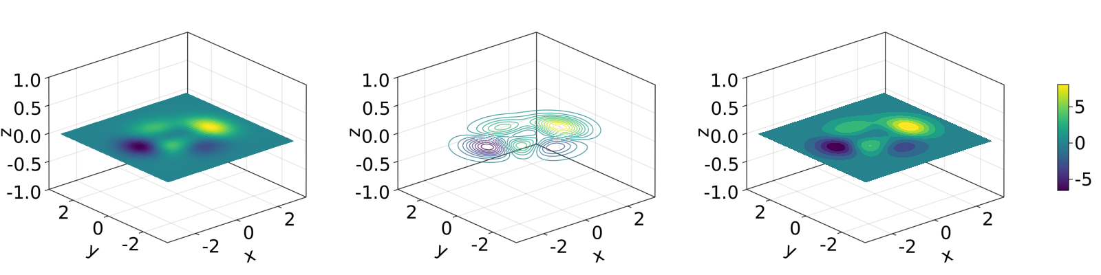

将这些绘图函数混合在一起也是非常简单的，如下所示：

using TestImages

function mixing_surface_contour3d_contour_and_contourf()
    img = testimage("coffee.png")
    x, y, z = peaks()
    cmap = :Spectral_11
    fig = Figure(resolution=(1200, 800), fontsize=26)
    ax1 = Axis3(fig[1, 1]; aspect=(1, 1, 1), elevation=pi / 6, xzpanelcolor=(:black, 0.75),
        perspectiveness=0.5, yzpanelcolor=:black, zgridcolor=:grey70,
        ygridcolor=:grey70, xgridcolor=:grey70)
    ax2 = Axis3(fig[1, 3]; aspect=(1, 1, 1), elevation=pi / 6, perspectiveness=0.5)
    hm = surface!(ax1, x, y, z; colormap=(cmap, 0.95), shading=true)
    contour3d!(ax1, x, y, z .+ 0.02; colormap=cmap, levels=20, linewidth=2)
    xmin, ymin, zmin = minimum(ax1.finallimits[])
    xmax, ymax, zmax = maximum(ax1.finallimits[])
    contour!(ax1, x, y, z; colormap=cmap, levels=20, transformation=(:xy, zmax))
    contourf!(ax1, x, y, z; colormap=cmap, transformation=(:xy, zmin))
    Colorbar(fig[1, 2], hm, width=15, ticksize=15, tickalign=1, height=Relative(0.35))
    # transformations into planes
    heatmap!(ax2, x, y, z; colormap=:viridis, transformation=(:yz, 3.5))
    contourf!(ax2, x, y, z; colormap=:CMRmap, transformation=(:xy, -3.5))
    contourf!(ax2, x, y, z; colormap=:bone_1, transformation=(:xz, 3.5))
    image!(ax2, -3 .. 3, -3 .. 2, rotr90(img); transformation=(:xy, 3.8))
    xlims!(ax2, -3.8, 3.8)
    ylims!(ax2, -3.8, 3.8)
    zlims!(ax2, -3.8, 3.8)
    fig
end
mixing_surface_contour3d_contour_and_contourf()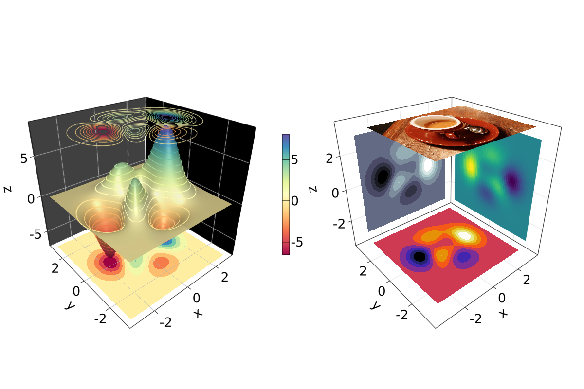

还不错，对吧？从这里也可以看出，任何的 heatmap， contour，contourf 和 image 都可以绘制在任何平面上。

5.7.3 arrows 和 streamplot

当想要知道给定变量的方向时，arrows 和 streamplot 会变得非常有用。 参见如下的示例¹⁸：

using LinearAlgebra

function arrows_and_streamplot_in_3d()
    ps = [Point3f(x, y, z) for x = -3:1:3 for y = -3:1:3 for z = -3:1:3]
    ns = map(p -> 0.1 * rand() * Vec3f(p[2], p[3], p[1]), ps)
    lengths = norm.(ns)
    flowField(x, y, z) = Point(-y + x * (-1 + x^2 + y^2)^2, x + y * (-1 + x^2 + y^2)^2,
        z + x * (y - z^2))
    fig = Figure(resolution=(1200, 800), fontsize=26)
    axs = [Axis3(fig[1, i]; aspect=(1, 1, 1), perspectiveness=0.5) for i = 1:2]
    arrows!(axs[1], ps, ns, color=lengths, arrowsize=Vec3f0(0.2, 0.2, 0.3),
        linewidth=0.1)
    streamplot!(axs[2], flowField, -4 .. 4, -4 .. 4, -4 .. 4, colormap=:plasma,
        gridsize=(7, 7), arrow_size=0.25, linewidth=1)
    fig
end
arrows_and_streamplot_in_3d()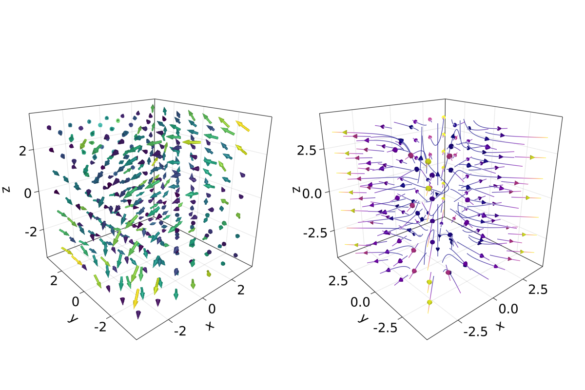

另外一些有趣的例子是 mesh(obj)，volume(x, y, z, vals) 和 contour(x, y, z, vals)。

5.7.4 mesh 和 volume

绘制网格在想要画出几何实体时很有用，例如 Sphere 或矩形这样的几何实体，即 FRect3D。 另一种在 3D 空间中可视化的方法是调用 volume 和 contour 函数，它们通过实现 光线追踪 来模拟各种光学效果。 例子如下：

using GeometryBasics

function mesh_volume_contour()
    # mesh objects
    rectMesh = FRect3D(Vec3f(-0.5), Vec3f(1))
    recmesh = GeometryBasics.mesh(rectMesh)
    sphere = Sphere(Point3f(0), 1)
    # https://juliageometry.github.io/GeometryBasics.jl/stable/primitives/
    spheremesh = GeometryBasics.mesh(Tesselation(sphere, 64))
    # uses 64 for tesselation, a smoother sphere
    colors = [rand() for v in recmesh.position]
    # cloud points for volume
    x = y = z = 1:10
    vals = randn(10, 10, 10)
    fig = Figure(resolution=(1600, 400))
    axs = [Axis3(fig[1, i]; aspect=(1, 1, 1), perspectiveness=0.5) for i = 1:3]
    mesh!(axs[1], recmesh; color=colors, colormap=:rainbow, shading=false)
    mesh!(axs[1], spheremesh; color=(:white, 0.25), transparency=true)
    volume!(axs[2], x, y, z, vals; colormap=Reverse(:plasma))
    contour!(axs[3], x, y, z, vals; colormap=Reverse(:plasma))
    fig
end
mesh_volume_contour()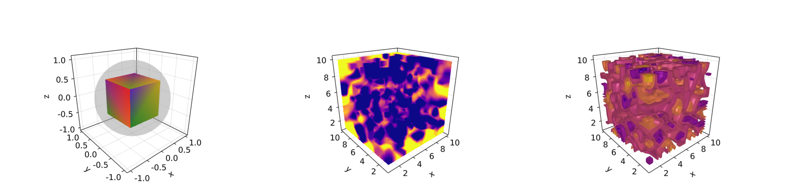

注意到透明球和立方体绘制在同一个坐标系中。 截至目前，我们已经包含了 3D 绘图的大多数用例。 另一个例子是 ?linesegments。

参考之前的例子，可以使用球体和矩形平面创建一些自定义图：

using GeometryBasics, Colors

首先为球体定义一个矩形网格，而且给每个球定义不同的颜色。 另外，可以将球体和平面混合在一张图里。下面的代码定义了所有必要的数据。

seed!(123)
spheresGrid = [Point3f(i,j,k) for i in 1:2:10 for j in 1:2:10 for k in 1:2:10]
colorSphere = [RGBA(i * 0.1, j * 0.1, k * 0.1, 0.75) for i in 1:2:10 for j in 1:2:10 for k in 1:2:10]
spheresPlane = [Point3f(i,j,k) for i in 1:2.5:20 for j in 1:2.5:10 for k in 1:2.5:4]
cmap = get(colorschemes[:plasma], LinRange(0, 1, 50))
colorsPlane = cmap[rand(1:50,50)]
rectMesh = FRect3D(Vec3f(-1, -1, 2.1), Vec3f(22, 11, 0.5))
recmesh = GeometryBasics.mesh(rectMesh)
colors = [RGBA(rand(4)...) for v in recmesh.position]

然后可使用如下方式简单地绘图：

function grid_spheres_and_rectangle_as_plate()
    fig = with_theme(theme_dark()) do
        fig = Figure(resolution=(1200, 800))
        ax1 = Axis3(fig[1, 1]; aspect=:data, perspectiveness=0.5, azimuth=0.72)
        ax2 = Axis3(fig[1, 2]; aspect=:data, perspectiveness=0.5)
        meshscatter!(ax1, spheresGrid; color = colorSphere, markersize = 1,
            shading=false)
        meshscatter!(ax2, spheresPlane; color=colorsPlane, markersize = 0.75,
            lightposition=Vec3f(10, 5, 2), ambient=Vec3f(0.95, 0.95, 0.95),
            backlight=1.0f0)
        mesh!(recmesh; color=colors, colormap=:rainbow, shading=false)
        limits!(ax1, 0, 10, 0, 10, 0, 10)
        fig
    end
    fig
end
grid_spheres_and_rectangle_as_plate()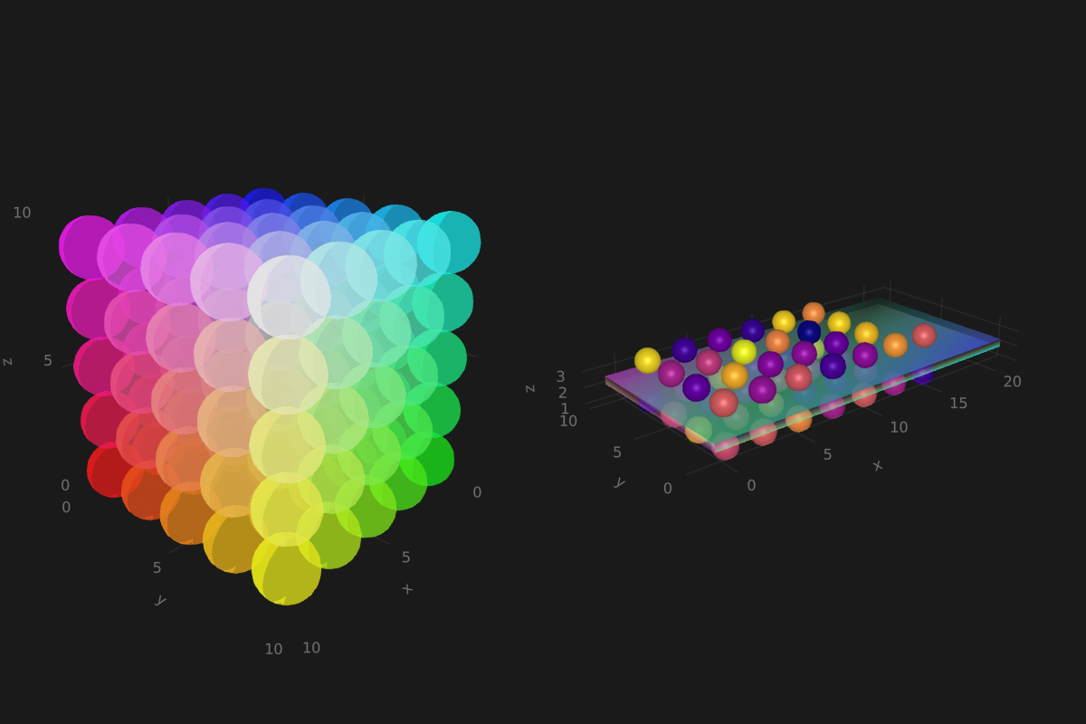

注意，右侧图中的矩形平面是半透明的，这是因为颜色函数 RGBA() 中定义了 alpha 参数。 矩形函数是通用的，因此很容易用来实现 3D 方块，而它又能用于绘制 3D 直方图。 参见如下的例子，我们将再次使用 peaks 函数并增加一些定义：

x, y, z = peaks(; n=15)
δx = (x[2] - x[1]) / 2
δy = (y[2] - y[1]) / 2
cbarPal = :Spectral_11
ztmp = (z .- minimum(z)) ./ (maximum(z .- minimum(z)))
cmap = get(colorschemes[cbarPal], ztmp)
cmap2 = reshape(cmap, size(z))
ztmp2 = abs.(z) ./ maximum(abs.(z)) .+ 0.15

其中方块的尺寸由 \(\delta x, \delta y\) 指定。 cmap2 用于指定每个方块的颜色而 ztmp2 用于指定每个方块的透明度。如下图所示。

function histogram_or_bars_in_3d()
    fig = Figure(resolution=(1200, 800), fontsize=26)
    ax1 = Axis3(fig[1, 1]; aspect=(1, 1, 1), elevation=π/6,
        perspectiveness=0.5)
    ax2 = Axis3(fig[1, 2]; aspect=(1, 1, 1), perspectiveness=0.5)
    rectMesh = FRect3D(Vec3f0(-0.5, -0.5, 0), Vec3f0(1, 1, 1))
    meshscatter!(ax1, x, y, 0*z, marker = rectMesh, color = z[:],
        markersize = Vec3f.(2δx, 2δy, z[:]), colormap = :Spectral_11,
        shading=false)
    limits!(ax1, -3.5, 3.5, -3.5, 3.5, -7.45, 7.45)
    meshscatter!(ax2, x, y, 0*z, marker = rectMesh, color = z[:],
        markersize = Vec3f.(2δx, 2δy, z[:]), colormap = (:Spectral_11, 0.25),
        shading=false, transparency=true)
    for (idx, i) in enumerate(x), (idy, j) in enumerate(y)
        rectMesh = FRect3D(Vec3f(i - δx, j - δy, 0), Vec3f(2δx, 2δy, z[idx, idy]))
        recmesh = GeometryBasics.mesh(rectMesh)
        lines!(ax2, recmesh; color=(cmap2[idx, idy], ztmp2[idx, idy]))
    end
    fig
end
histogram_or_bars_in_3d()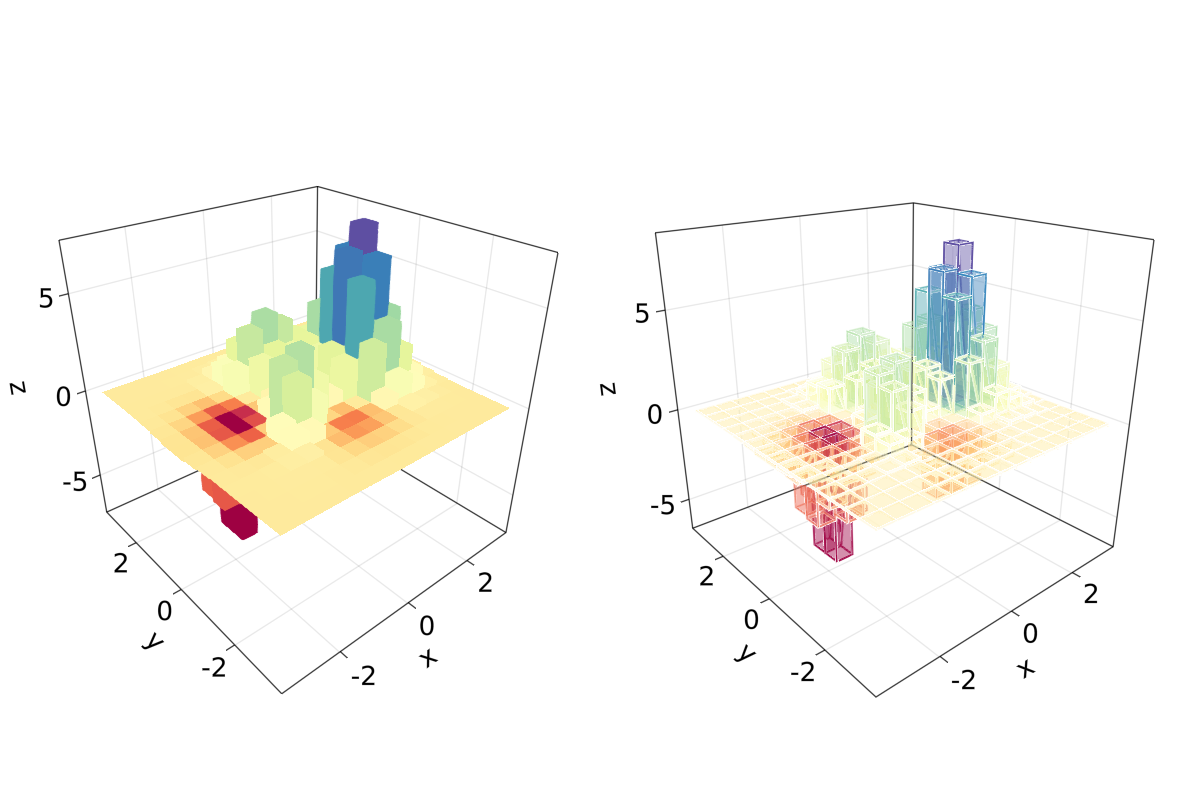

应注意到，也可以在 mesh 对象上调用 lines 或 wireframe。

5.7.5 填充的线和带

在最终的例子中， 我们将展示如何使用 band和一些 linesegments 填充 3D 图中的曲线：

function filled_line_and_linesegments_in_3D()
    xs = LinRange(-3, 3, 10)
    lower = [Point3f(i, -i, 0) for i in LinRange(0, 3, 100)]
    upper = [Point3f(i, -i, sin(i) * exp(-(i + i))) for i in range(0, 3, length=100)]
    fig = Figure(resolution=(1200, 800))
    axs = [Axis3(fig[1, i]; elevation=pi/6, perspectiveness=0.5) for i = 1:2]
    band!(axs[1], lower, upper, color=repeat(norm.(upper), outer=2), colormap=:CMRmap)
    lines!(axs[1], upper, color=:black)
    linesegments!(axs[2], cos.(xs), xs, sin.(xs), linewidth=5, color=1:length(xs))
    fig
end
filled_line_and_linesegments_in_3D()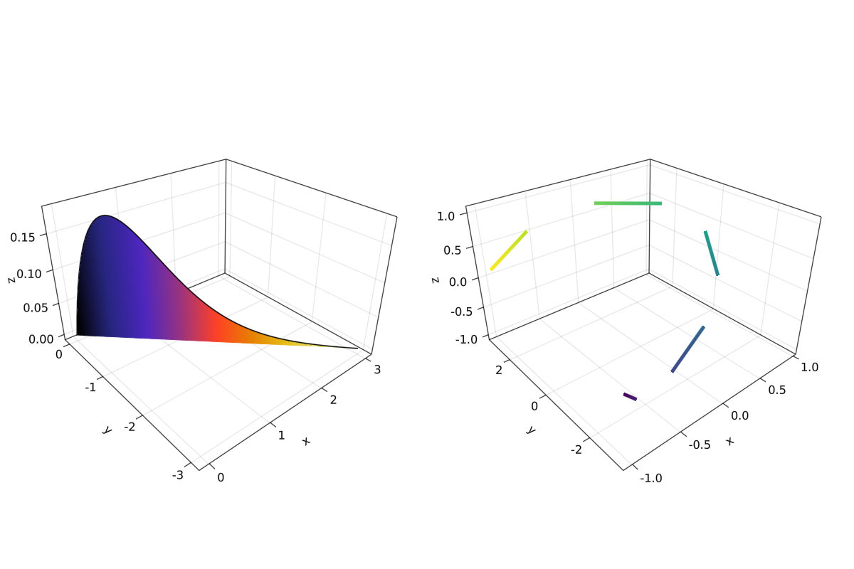

最后，我们的3D绘图之旅到此结束。 你可以将我们这里展示的一切结合起来，去创造令人惊叹的 3D 图！