Participant: Kenta Sato (@bicycle1885)
Mentor: Daniel C. Jones (@dcjones)
Thanks to a grant from the Gordon and Betty Moore Foundation, I've enjoyed the Julia Summer of Code 2015 program administered by the NumFOCUS and a travel to the JuliaCon 2015 at Boston. During this program, I have created several packages about data structures and algorithms for sequence analysis, mainly targeted for bioinformatics. Even though Julia had lots of practical packages for numerical computing on floating-point numbers, it lacked efficient and compact data structures that are fundamental in bioinformatics.
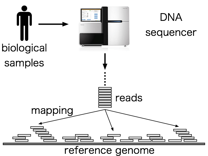
Recent development of high-throughput DNA sequencers has enabled to sequence massive numbers of DNA fragments (known as reads) from biological samples within a day. The first step of sequence analysis is locating positions of these fragments in other long reference sequence, then we can detect genetic variants or gene expressions based on the result. This step is called sequence mapping or aligning, and because reference sequences are most commonly genome-scale (about 3.2 billions length for human), a full-text search index is used to speed up this alignment process. This kind of full-text search index is implemented in many bioinformatics tools, most notably bowtie2 and BWA, whose papers are cited thousands of times.
The main focus of my project was creating a full-text search index in Julia that is easy to use and efficient in practical applications. In the course towards this destination, I've created several packages that are useful as a building block for other data structures. I'm going to introduce you these packages in this post.
IntArrays.jl
IntArrays.jl is a package for arrays of unsigned integer. So, is it useful? Yes, it is! This is because the IntArray type implemented in this package can store integers as small space as possible. The IntArray type has a type parameter w that represents the number of bits required to encode elements in an array. For example, if each element is an integer between 0 and 3, you only need to use two bits to encode it and w can be set to 2 or greater. These 2-bit integers are packed into a buffer and therefore the array consumes only one fourth of the space compared to the usual array. The following is a case of a byte sequence of [0x01, 0x03, 0x02, 0x00]:
    index:                           1          2          3          4
    byte sequence (hex):          0x01       0x03       0x02       0x00
    byte sequence (bin):    0b00000001 0b00000011 0b00000010 0b00000000
    packed sequence (w=2):          01         11         10         00
    in-memory layout:         00101101
The full type definition is IntArray{w,T,n}, where w is the number of bits for each element as I explained, T is the type of elements, and n is the dimension of the array. This type is a subtype of the AbstractArray{T,n} and will behave like a familiar array; allocation, random access and update are supported. IntVector and IntMatrix are also defined as type aliases like Vector and Matrix, respectively.
Here is an example:
julia> IntArray{2,UInt8}(2, 3)
2x3 IntArrays.IntArray{2,UInt8,2}:
 0x00  0x00  0x01
 0x00  0x00  0x03

julia> array = IntVector{2,UInt8}(6)
6-element IntArrays.IntArray{2,UInt8,1}:
 0x00
 0x00
 0x03
 0x03
 0x02
 0x00

julia> array[1] = 0x02
0x02

julia> array
6-element IntArrays.IntArray{2,UInt8,1}:
 0x02
 0x00
 0x03
 0x03
 0x02
 0x00

julia> sort!(array)
6-element IntArrays.IntArray{2,UInt8,1}:
 0x00
 0x00
 0x02
 0x02
 0x03
 0x03
And the memory footprint of IntArray is much smaller:
julia> sizeof(IntVector{2,UInt8}(1_000_000))
250000

julia> sizeof(Vector{UInt8}(1_000_000))
1000000
Since packing and unpacking integers in a buffer require additional operations, there are overheads in operations and IntArray is often slower than Array. I've tried to keep this discrepancy as small as possible, but the IntArray is about 4-5 times slower when sorting it:
julia> array = rand(0x00:0x03, 2^24);

julia> sort(array); @time sort(array);
  0.488779 seconds (8 allocations: 16.000 MB)

julia> iarray = IntVector{2}(array);

julia> sort(iarray); @time sort(iarray);
  2.290878 seconds (18 allocations: 4.001 MB)
If you have a great idea to improve the performance, please let me know!
IndexableBitVectors.jl
The next package is IndexableBitVectors.jl. You must be familiar with the BitVector type in the standard library; types defined in my package is a static but indexable version of it. Here "indexable" means that a query to ask the number of bits between an arbitrary range can be answered in constant time. If you are already familiar with succinct data structures, you may know this is an important building block of other succinct data structures like wavelet trees, LOUDS, etcetera.
The package exports two variants of such bit vectors: SucVector and RRR. SucVector is simpler and faster than RRR, but RRR is compressible and will be smaller if 0/1 bits are localized in a bit vector. Both types split a bit vector into blocks and cache the number of bits up to the position. In SucVector, the extra space is about 1/4 bits per bit, so it will become ~25% larger than the original bit vector.
The most important query operation over these data structures would be the rank1(bv, i) query, which counts the number of 1 bits within bv[1:i]. Owing to the cached bit counts, we can finish the rank operation in constant time:
julia> using IndexableBitVectors

julia> bv = bitrand(2^30);

julia> function myrank1(bv, i)  # count ones by loop
           r = 0
           for j in 1:i
               r += bv[j]
           end
           return r
       end
myrank1 (generic function with 1 method)

julia> myrank1(bv, 2^29); @time myrank1(bv, 2^29);
  0.714866 seconds (6 allocations: 192 bytes)

julia> sbv = SucVector(bv);

julia> rank1(sbv, 2^29); @time rank1(sbv, 2^29);  # much faster!
  0.000003 seconds (6 allocations: 192 bytes)

julia> rrr = RRR(bv);

julia> rank1(rrr, 2^29); @time rank1(rrr, 2^29);  # much faster, too!
  0.000004 seconds (6 allocations: 192 bytes)
The select1(bv, j) query is also useful in many cases, which locates the j-th 1 bit in the bit vector bv. For example, if a set of positive integers is represented in this bit vector, you can efficiently query the j-th smallest member in the set.
Let's see the internal representation of SucVector to understand the magic. A bit vector is separated into large blocks:
type SucVector <: AbstractIndexableBitVector
    blocks::Vector{Block}
    len::Int
end
Each large block contains 256 bits and consists of four small blocks which contain 64 bits respectively, a large block stores global 1s' count up to the starting position of it and a small block stores local 1s' count staring from the beginning position of its parent large block. Bits itself are stored in four bit chunks corresponding to small blocks:
immutable Block
    # large block
    large::UInt32
    # small blocks
    #   the first small block is used for 8-bit extension of the large block
    #   hence, 40 (= 32 + 8) bits are available in total
    smalls::NTuple{4,UInt8}
    # bit chunks (64bits × 4 = 256bits)
    chunks::NTuple{4,UInt64}
end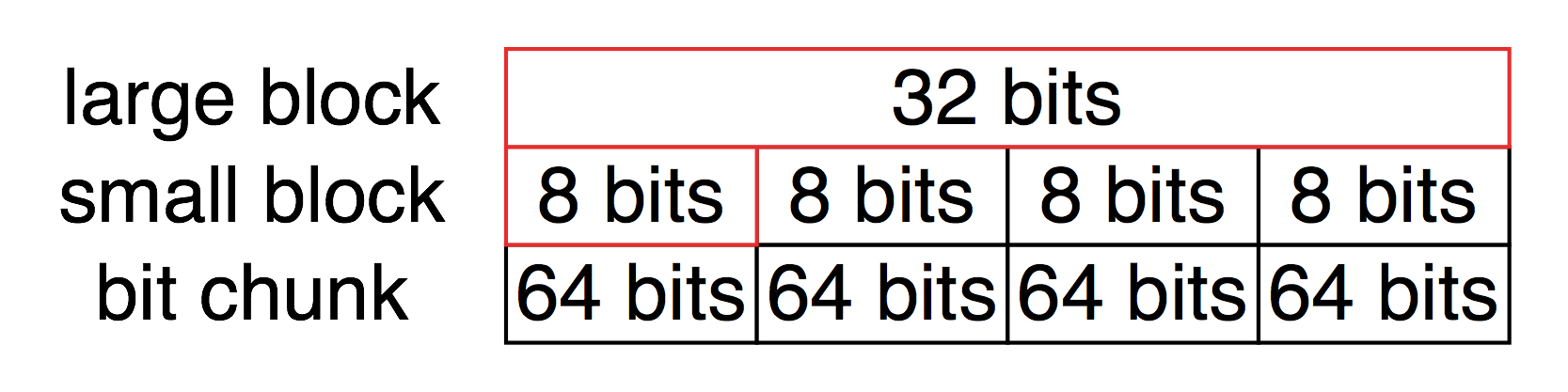
Since the bit count of the first small block is always zero, we can exploit this space to extend the cache of the large block (red frame). When running the rank1(bv, i) query, it first picks a large and small block pair that the i-th bit belongs to and then adds their cached bit counts, finally counts remaining 1 bits in a chunk on the fly.
As I mentioned, this data structure can be used as a building block of various data structures. The next package I'm going to introduce is one of them.
WaveletMatrices.jl
You may already know about the wavelet tree, which supports the rank and select queries like SucVector and RRR, but elements are not restricted to 0/1 bits. In fact, the rank and select queries are available on arbitrary unsigned integers. The wavelet tree can be thought as a generalization of indexable bit vectors in this respect. What I've implemented is not the well-known wavelet tree, a variant of it called "wavelet matrix". You can find an implementation and a link to a paper at WaveletMatrices.jl. According to the authors of the paper, the wavelet matrix is "simpler to build, simpler to query, and faster in practice than the levelwise wavelet tree".
The WaveletMatrix type takes three type parameters: w, T, and B. w and T are analogous to those of IntArray{w,T,n}, and B is a type of indexable bit vector.
julia> using WaveletMatrices

julia> wm = WaveletMatrix{2}([0x00, 0x01, 0x02, 0x03])
4-element WaveletMatrices.WaveletMatrix{2,UInt8,IndexableBitVectors.SucVector}:
 0x00
 0x01
 0x02
 0x03

julia> wm[3]
0x02

julia> rank(0x02, wm, 2)
0

julia> rank(0x02, wm, 3)
1

julia> xs = rand(0x00:0x03, 2^16);

julia> wm = WaveletMatrix{2}(xs);  # 2-bit encoding

julia> sum(xs[1:2^15] .== 0x03)
8171

julia> rank(0x03, wm, 2^15)
8171
The details of the data structure and algorithms are relatively simple but beyond the scope of this post. For people who are interested in this data structure, the paper I mentioned above and my implementation would be helpful. There are more operations that the wavelet matrix can run efficiently and those operations will be added in the future.
FMIndexes.jl
80% of sequence analysis in bioinformatics is about sequence search, which includes pattern search, homologous gene search, genome comparison, short-read mapping, and so on. The FM-Index is often regarded as one of the most efficient indices for full-text search, and I've implemented it in the FMIndexes.jl package. Thanks to the packages I've introduced so far, the code of it looks really simple. For example, counting the number of occurrences of a given pattern in a text can be written as follows (slightly simplified for explanatory purpose):
function count(query, index::FMIndex)
    sp, ep = 1, length(index)
    # backward search
    i = length(query)
    while sp ≤ ep && i ≥ 1
        char = convert(UInt8, query[i])
        c = index.count[char+1]
        sp = c + rank(char, index.bwt, sp - 1) + 1
        ep = c + rank(char, index.bwt, ep)
        i -= 1
    end
    return length(sp:ep)
end
A unique property of the FM-Index is that an index itself is just a permutation of characters of an original text and counts of characters contained in it. This permutation is called Burrows-Wheeler transform (also known as BWT), and the permuted text is stored in a wavelet matrix (or a wavelet tree) in order to efficiently count the number of characters within a specific region. Therefore, the space required to index a text is often smaller than that of other full-text indices (actually, in practice, efficiently finding positions of a query needs auxiliary data as well). Moreover, this transform is bijective, and thus the original text can be restored from an index.
Building an index for full-text search is ridiculously simple: just passing a sequence to a constructor:
julia> using FMIndexes

julia> fmindex = FMIndex("abracadabra");
The FMIndex type supports two main queries: count and locate. The count(query, index) query literally counts the number of occurrences of the query string and the locate(query, index) locates starting positions of the query. In order to restore the original text, you can use the restore function. Here is a simple usage:
julia> count("a", fmindex)
5

julia> count("abra", fmindex)
2

julia> locate("a", fmindex) |> collect
5-element Array{Any,1}:
 11
  8
  1
  4
  6

julia> locate("abra", fmindex) |> collect
2-element Array{Any,1}:
 8
 1

julia> bytestring(restore(fmindex))
"abracadabra"
As an example, for bioinformaticians, let's try several queries on a chromosome. You also need to install the Bio.jl package to efficiently parse a FASTA file. The next script reads a chromosome from a FASTA file, build an FM-Index, and then serialize it into a file for later use (I love the serializers of Julia, they are available for free!):
index.jl
using Bio.Seq
using IntArrays
using FMIndexes

# encode a DNA sequence with 3-bit unsigned integers;
# this is because a reference genome has five nucleotides: A/C/G/T/N.
function encode(seq)
    encoded = IntVector{3,UInt8}(length(seq))
    for i in 1:endof(seq)
        encoded[i] = convert(UInt8, seq[i])
    end
    return encoded
end

# read a chromosome from a FASTA file
filepath = ARGS[1]
record = first(open(filepath, FASTA))
println(record.name, ": ", length(record.seq), "bp")
# build an FM-Index
fmindex = FMIndex(encode(record.seq))
# save it in a file
open(string(filepath, ".index"), "w+") do io
    serialize(io, fmindex)
end
OK, then create an index for chromosome 22 of human (you can download it from here):
$ julia4 index.jl chr22.fa
chr22: 50818468bp
$ ls -lh chr22.fa.index
-rw-r--r--+ 1 kenta  staff    74M  9 26 06:30 chr22.fa.index
After construction finished (this will take several minutes), read the index in REPL:
julia> using FMIndexes

julia> fmindex = open(deserialize, "chr22.fa.index");
Now that you can execute queries to search a DNA fragment:
julia> using Bio.Seq

julia> count(dna"GACTTTCAC", fmindex)  # this DNA fragment hits at 111 locations
111

julia> count(dna"GACTTTCACTTT", fmindex)  # this hits at 3 locations
3

julia> locate(dna"GACTTTCACTTT", fmindex) |> collect  # the loci of these hits
3-element Array{Any,1}:
 36253071
 47308573
 34159872

julia> count(dna"GACTTTCACTTTCCC", fmindex)  # found a unique hit!
1

julia> locate(dna"GACTTTCACTTTCCC", fmindex) |> collect
1-element Array{Any,1}:
 36253071

julia> @time locate(dna"GACTTTCACTTTCCC", fmindex);  # this can be located in 32 μs!
  0.000032 seconds (5 allocations: 192 bytes)
This locus, chr22:36253071, is the starting position of the APOL1 gene.
Applications
My aim of having created these packages was to prove that it is practicable to implement high-performance data structures for bioinformatics in Julia. I'm pretty sure that it is true, but it may be skeptical to others. So, I'm going to prove it by writing useful and performant applications using these packages. Now I'm working on FMM.jl, which aligns massive amounts of DNA fragments to a genome sequence using the FM-Index and other algorithms. This is still a work in progress, there would be many bugs and unusual cases I should care about, but its performance is not so bad compared to other implementations.
The BioJulia project is also under active development. The packages I made are intended to work with the Bio.jl package. If you are interested in the BioJulia project, we really welcome your contributions!