GSoC 2017 Project: Hamiltonian Indirect Inference
Bayesian_Examples.jl
This is a writeup of my project for the Google Summer of Code 2017. The associated repository contains examples of estimating various models. In addition to this repository, I have collaborated in HamiltonianABC and its branches as part of the GSOC 2017.
GSOC 2017 project: Hamiltonian Monte Carlo and pseudo-Bayesian Indirect Likelihood
This summer I have had the opportunity to participate in the Google Summer of Code program. My project was in the Julia language and the main goal was to implement Indirect Inference (A. A. Smith 1993; A. Smith 2008) to overcome the typically arising issues (such as intractable or costly to compute likelihoods) when estimating models using likelihood-based methods. Hamiltonian Monte Carlo was expected to result in a more efficient sampling process.
Under the mentorship of Tamás K. Papp, I completed a major revision of Bayesian estimation methods using Indirect Inference (II) and Hamiltonian Monte Carlo. I also got familiar with using git, opening issues, creating a repository among others.
Here I introduce the methods with a bit of context, and dicuss an example more extensively.
Parametric Bayesian Indirect Likelihood for the Full Data
Usually when we face an intractable likelihood or a likelihood that would be extremely costly to calculate, we have the option to use an alternative auxiliary model to extract and estimate the parameters of interest. These alternative models should be easier to deal with. Drovandi et al. reviews a collection of parametric Bayesian Indirect Inference (pBII) methods, I focused on the parametric Bayesian Indirect Likelihood for the Full Data (pdBIL) method proposed by Gallant and McCulloch (2009). The pdBIL uses the likelihood of the auxiliary model as a substitute for the intractable likelihood. The pdBIL does not compare summary statistics, instead works in the following way:
First the data is generated, once we have the data, we can estimate the parameters of the auxiliary model. Then, the estimated parameters are put into the auxiliary likelihood with the observed/generated data. Afterwards we can use this likelihood in our chosen Bayesian method i.e. MCMC.
To summarize the method, first we have the parameter vector $\theta$ and the observed data y. We would like to calculate the likelihood of $\ell(\theta|y)$, but it is intractable or costly to compute. In this case, with pdBIL we have to find an auxiliary model (A) that we use to approximate the true likelihood in the following way:
- First we have to generate points, denote with x* from the data generating process with the previously proposed parameters $\theta$.
-
Then we compute the MLE of the auxiliary likelihood under x to get the parameters denoted by $\phi$. \
- Under these parameters \phi, we can now compute the likelihood of $\ell_{A}(y|\phi). It is desirable to have the auxiliary likelihood as close to the true likelihood as possible, in the sense of capturing relevant aspects of the model and the generated data.
First stage of my project
In the first stage of my project I coded two models from Drovandi et al. using pdBIL. After calculating the likelihood of the auxiliary model, I used a Random Walk Metropolis-Hastings MCMC to sample from the target distribution, resulting in Toy models. In this stage of the project, the methods I used were well-known. The purpose of the replication of the toy models from Drovandi et al. was to find out what issues we might face later on and to come up with a usable interface. This stage resulted in HamiltonianABC (collaboration with Tamás K. Papp).
Second stage of my project
After the first stage, I worked through Betancourt (2017) and did a code revision for Tamás K. Papp’s DynamicHMC.jl which consisted of checking the code and its comparison with the paper. In addition to using the Hamiltonian Monte Carlo method, the usage of the forward mode automatic differentiation of the ForwardDiff package was the other main factor of this stage. The novelty of this project was to find a way to fit every component together in a way to get an efficient estimation out of it. The biggest issue was to define type-stable functions such that to accelerate the sampling process.
Stochastic Volatility model
After the second stage, I coded economic models for the DynamicHMC.jl. The Stochastic Volatility model is one of them. In the following section, I will go through the set up.
The continuous-time version of the Ornstein-Ulenbeck Stochastic - volatiltiy model describes how the return at time t has mean zero and its volatility is governed by a continuous-time Ornstein-Ulenbeck process of its variance. The big fluctuation of the value of a financial product imply a varying volatility process. That is why we need stochastic elements in the model. As we can access data only in discrete time, it is natural to take the discretization of the model.
The discrete-time version of the Ornstein-Ulenbeck Stochastic - volatility model:
The discrete-time version was used as the data-generating process. Where yₜ denotes the logarithm of return, $x_{t}$ is the logarithm of variance, while $\epsilon_{t}$ and $\nu_{t}$ are unobserved noise terms.
For the auxiliary model, we used two regressions. The first regression was an AR(2) process on the first differences, the second was also an AR(2) process on the original variables in order to capture the levels.
"""
    lag_matrix(xs, ns, K = maximum(ns))

Matrix with differently lagged xs.
"""
function lag_matrix(xs, ns, K = maximum(ns))
    M = Matrix{eltype(xs)}(length(xs)-K, maximum(ns))
    for i ∈ ns
        M[:, i] = lag(xs, i, K)
    end
    M
end

"first auxiliary regression y, X, meant to capture first differences"
function yX1(zs, K)
    Δs = diff(zs)
    lag(Δs, 0, K), hcat(lag_matrix(Δs, 1:K, K), ones(eltype(zs), length(Δs)-K), lag(zs, 1, K+1))
end

"second auxiliary regression y, X, meant to capture levels"
function yX2(zs, K)
    lag(zs, 0, K), hcat(ones(eltype(zs), length(zs)-K), lag_matrix(zs, 1:K, K))
end
The AR(2) process of the first differences can be summarized by: \ Given a series Y, it is the first difference of the first difference. The so called “change in the change” of Y at time t. The second difference of a discrete function can be interpreted as the second derivative of a continuous function, which is the “acceleration” of the function at a point in time t. In this model, we want to capture the “acceleration” of the logarithm of return.
The AR(2) process of the original variables is needed to capture the effect of $\rho$. It turned out that the impact of ρ was rather weak in the AR(2) process of the first differences . That is why we need a second auxiliary model.
I will now describe the required steps for the estimation of the parameters of interest in the stochastic volatility model with the Dynamic Hamiltonian Monte Carlo method. First we need a callable Julia object which gives back the logdensity and the gradient in DiffResult type. After that, we write a function that computes the density, then we calculate its gradient using the ForwardDiff package in a wrapper function.
Required packages for the StochasticVolatility model:
using ArgCheck
using Distributions
using Parameters
using DynamicHMC
using StatsBase
using Base.Test
using ContinuousTransformations
using DiffWrappers
import Distributions: Uniform, InverseGamma
- First, we define a structure. This structure should contain the observed data, the priors, the shocks and the transformation performed on the parameters, but the components may vary depending on the estimated model.
struct StochasticVolatility{T, Prior_ρ, Prior_σ, Ttrans}
    "observed data"
    ys::Vector{T}
    "prior for ρ (persistence)"
    prior_ρ::Prior_ρ
    "prior for σ_v (volatility of volatility)"
    prior_σ::Prior_σ
    "χ^2 draws for simulation"
    ϵ::Vector{T}
    "Normal(0,1) draws for simulation"
    ν::Vector{T}
    "Transformations cached"
    transformation::Ttrans
end
After specifying the data generating function and a couple of facilitator and additional functions for the particular model (whole module can be found in src folder), we can make the model structure callable, returning the log density. The logjac is needed because of the transformation we make on the parameters.
function (pp::StochasticVolatility)(θ)
    @unpack ys, prior_ρ, prior_σ, ν, ϵ, transformation = pp
    ρ, σ = transformation(θ)
    logprior = logpdf(prior_ρ, ρ) + logpdf(prior_σ, σ)
    N = length(ϵ)

    # Generating xs, which is the latent volatility process

    xs = simulate_stochastic(ρ, σ, ϵ, ν)
    Y_1, X_1 = yX1(xs, 2)
    β₁ = qrfact(X_1, Val{true}) \ Y_1
    v₁ = mean(abs2,  Y_1 - X_1*β₁)
    Y_2, X_2 = yX2(xs, 2)
    β₂ = qrfact(X_2, Val{true}) \ Y_2
    v₂ = mean(abs2,  Y_2 - X_2*β₂)
    # We work with first differences
    y₁, X₁ = yX1(ys, 2)
    log_likelihood1 = sum(logpdf.(Normal(0, √v₁), y₁ - X₁ * β₁))
    y₂, X₂ = yX2(ys, 2)
    log_likelihood2 = sum(logpdf.(Normal(0, √v₂), y₂ - X₂ * β₂))
    logprior + log_likelihood1 + log_likelihood2 + logjac(transformation, θ)
end
We need the transformations because the parameters are in the proper subset of $\Re^{n}$, but we want to use $\Re^{n}$. The ContinuousTransformation package is used for the transformations. We save the transformations such that the callable object stays type-stable which makes the process faster.
$\nu$ and $\epsilon$ are random variables which we use after the transformation to simulate observation points. This way the simulated variables are continuous in the parameters and the posterior is differentiable.
Given the defined functions, we can now start the estimation and sampling process:
RNG = Base.Random.GLOBAL_RNG
# true parameters and observed data
ρ = 0.8
σ = 0.6
y = simulate_stochastic(ρ, σ, 10000)
# setting up the model
model = StochasticVolatility(y, Uniform(-1, 1), InverseGamma(1, 1), 10000)
# we start the estimation process from the true values
θ₀ = inverse(model.transformation, (ρ, σ))
# wrap for gradient calculations
fgw = ForwardGradientWrapper(model, θ₀)
# sampling
sample, tuned_sampler = NUTS_tune_and_mcmc(RNG, fgw, 5000; q = θ₀)
The following graphs show the results for the parameters:
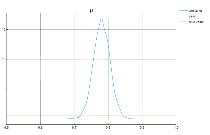
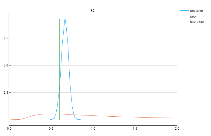
Analysing the graphs above, we can say that the posterior values are in rather close to the true values. Also worth mentioning that the priors do not affect the posterior values.
Problems that I have faced during GSOC
1) Difficult auxiliary model
- The true model was the g-and-k quantile function described by Rayner and MacGillivray (2002).
- The auxiliary model was a three component normal mixture model.
We faced serious problems with this model. \ First of all, I coded the MLE of the finite component normal mixture model, which computes the means, variances and weights of the normals given the observed data and the desired number of mixtures. With the g-and-k quantile function, I experienced the so called “isolation”, which means that one observation point is an outlier getting weight 1, the other observed points get weight $\theta$, which results in variance equal to $\theta$. There are ways to disentangle the problem of isolation, but the parameters of interests still did not converge to the true values. There is work to be done with this model.
2) Type-stability issues
To use the automatic differentiation method efficiently, I had to code the functions to be type-stable, otherwise the sampling functions would have taken hours to run. See the following example:
- This is not type-stable
function simulate_stochastic(ρ, σ, ϵs, νs) N = length(ϵs) @argcheck N == length(νs) xs = Vector(N) for i in 1:N xs[i] = (i == 1) ? νs[1]*σ*(1 - ρ^2)^(-0.5) : (ρ*xs[i-1] + σ*νs[i]) end xs + log.(ϵs) + 1.27 end - This is type-stable
function simulate_stochastic(ρ, σ, ϵs, νs)
  N = length(ϵs)
  @argcheck N == length(νs)
  x₀ = νs[1]*σ*(1 - ρ^2)^(-0.5)
    xs = Vector{typeof(x₀)}(N)
    for i in 1:N
        xs[i] = (i == 1) ? x₀ : (ρ*xs[i-1] + σ*νs[i])
    end
  xs + log.(ϵs) + 1.27
end
Future work
-
More involved models
-
Solving isolation in the three component normal mixture model
-
Updating shocks in every iteration
-
Optimization
References
- Betancourt, M. (2017). A Conceptual Introduction to Hamiltonian Monte Carlo.
- Drovandi, C. C., Pettitt, A. N., & Lee, A. (2015). Bayesian indirect inference using a parametric auxiliary model.
- Gallant, A. R. and McCulloch, R. E. (2009). On the Determination of General Scientific Models With Application to Asset Pricing
- Martin, G. M., McCabe, B. P. M., Frazier, D. T., Maneesoonthorn, W. and Robert, C. P. (2016). Auxiliary Likelihood-Based Approximate Bayesian Computation in State Space Models
- Rayner, G. D. and MacGillivray, H. L. (2002). Numerical maximum likelihood estimation for the g-and-k and generalized g-and-h distributions. In: Statistical Computation 12 57–75.
- Smith, A. A. (2008). “Indirect inference”. In: New Palgrave Dictionary of Economics, 2nd Edition (forthcoming).
- Smith, A. A. (1993). “Estimating nonlinear time-series models using simulated vector autoregressions”. In: Journal of Applied Econometrics 8.S1.